概念
通常我们对于biomarker的预测模型会用ROC曲线来评价其性能,但是对于一些生存资料数据的预测模型或者需要加入时间因素,则会使用时间依赖(time dependent)的ROC曲线
传统的ROC曲线分析方法认为个体的事件(疾病)状态和markers是随着时间的推移而固定的,但在临床流行病学研究中,疾病状态和markers都是随着时间的推移而变化的(即time-to-event outcomes)。早期无病的个体由于研究随访时间较长,可能较晚发病,而且其markers可能在随访期间较基线发生变化。如果使用传统的ROC会忽略疾病状态或markers的时间依赖性,此时用随时间变化的time-dependent ROC(时间相依ROC)比较合适。 来自---真实世界大数据分析系列|ROC曲线与Time-dependent ROC 曲线
对于常规的ROC曲线,在之前的笔记(理解ROC和AUC)中对其原理做了简单的介绍,而time-dependent ROC曲线的原理与常规的ROC曲线比较类似,前者相比后者多了时间因素,以便我们可以根据不同时间节点绘制不同的ROC曲线
本质上ROC曲线可以根据灵敏度和特异度两个指标来绘制的,所以我们通过比较常规的ROC曲线和time-dependent的ROC曲线对于灵敏度和特异度的计算公式即可明白两者的差别了
公式可以参考真实世界大数据分析系列|ROC曲线与Time-dependent ROC 曲线和时间依赖性ROC曲线(一),虽然两者公式的表现形式不同,但是细想下,其实是同一个意思
上述说的是Cumulative case/dynamic control ROC,另外还有一种Incident case/dynamic control ROC(似乎不太常见),可参考:Time-dependent ROC for Survival Prediction Models in R
实现方式
对于R中time-dependent ROC的实现方式,我一般会用timeROC和survivalROC包,当然还有其他的包(听说。。未尝试过),如:tdROC, timereg, risksetROC和survAUC
timeROC包相比survivalROC包会多计算个AUC的置信区间
若数据是生存资料数据,那么还会有不同的处理删除(censoring)方式,如Kaplan-Meier(KM), Cox model以及NNE(Nearest Neighbor Estimation)等等
下面以survivalROC包的mayo数据为例,其中mayoscore5和mayoscore4是两个marker,ROC曲线的绘制则用timeROC包
library(timeROC)
library(survival)

data(mayo)

time_roc_res <- timeROC(
  T = mayo$time,
  delta = mayo$censor,
  marker = mayo$mayoscore5,
  cause = 1,
  weighting="marginal",
  times = c(3 * 365, 5 * 365, 10 * 365),
  ROC = TRUE,
  iid = TRUE
)
计算AUC值及其置信区间
> time_roc_res$AUC
   t=1095    t=1825    t=3650
0.8982790 0.9153621 0.8576153
查看AUC的95%置信区间
> confint(time_roc_res, level = 0.95)$CI_AUC
        2.5% 97.5%
t=1095 85.01 94.64
t=1825 87.42 95.65
t=3650 79.38 92.14
绘制time-dependent ROC曲线
简单绘制下time-dependent ROC曲线(这里的plot函数对应的是timeROC::plot.ipcwsurvivalROC函数)
plot(time_roc_res, time=3 * 365, col = "red", title = FALSE)
plot(time_roc_res, time=5 * 365, add=TRUE, col="blue")
plot(time_roc_res, time=10 * 365, add=TRUE, col="green")
legend("bottomright",c("3 Years" ,"5 Years", "10 Years"),
       col=c("red", "blue", "green"), lty=1, lwd=2)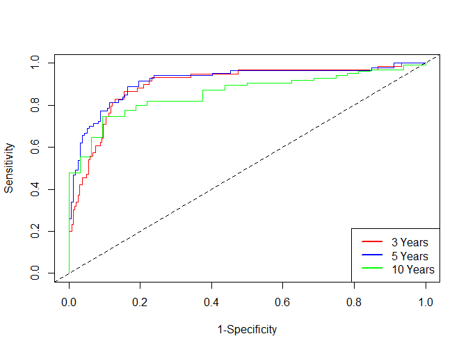
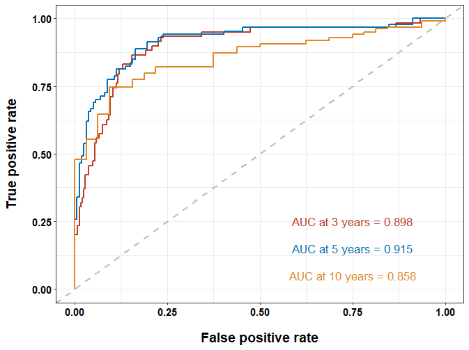
也可以通过修改在再美观点,如:
time_ROC_df <- data.frame(
  TP_3year = time_roc_res$TP[, 1],
  FP_3year = time_roc_res$FP[, 1],
  TP_5year = time_roc_res$TP[, 2],
  FP_5year = time_roc_res$FP[, 2],
  TP_10year = time_roc_res$TP[, 3],
  FP_10year = time_roc_res$FP[, 3]
)
library(ggplot2)
ggplot(data = time_ROC_df) +
  geom_line(aes(x = FP_3year, y = TP_3year), size = 1, color = "#BC3C29FF") +
  geom_line(aes(x = FP_5year, y = TP_5year), size = 1, color = "#0072B5FF") +
  geom_line(aes(x = FP_10year, y = TP_10year), size = 1, color = "#E18727FF") +
  geom_abline(slope = 1, intercept = 0, color = "grey", size = 1, linetype = 2) +
  theme_bw() +
  annotate("text",
           x = 0.75, y = 0.25, size = 4.5,
           label = paste0("AUC at 3 years = ", sprintf("%.3f", time_roc_res$AUC[[1]])), color = "#BC3C29FF"
  ) +
  annotate("text",
           x = 0.75, y = 0.15, size = 4.5,
           label = paste0("AUC at 5 years = ", sprintf("%.3f", time_roc_res$AUC[[2]])), color = "#0072B5FF"
  ) +
  annotate("text",
           x = 0.75, y = 0.05, size = 4.5,
           label = paste0("AUC at 10 years = ", sprintf("%.3f", time_roc_res$AUC[[3]])), color = "#E18727FF"
  ) +
  labs(x = "False positive rate", y = "True positive rate") +
  theme(
    axis.text = element_text(face = "bold", size = 11, color = "black"),
    axis.title.x = element_text(face = "bold", size = 14, color = "black", margin = margin(c(15, 0, 0, 0))),
    axis.title.y = element_text(face = "bold", size = 14, color = "black", margin = margin(c(0, 15, 0, 0)))
  )
比较两个time-dependent AUC
按照上述方式对mayoscore4marker做类似的分析
time_roc_res2 <- timeROC(
  T = mayo$time,
  delta = mayo$censor,
  marker = mayo$mayoscore4,
  cause = 1,
  weighting="marginal",
  times = c(3 * 365, 5 * 365, 10 * 365),
  ROC = TRUE,
  iid = TRUE
)
> time_roc_res2$AUC
   t=1095    t=1825    t=3650
0.8454230 0.8285379 0.7667952 然后通过compare函数进行比较,并输出矫正后的P值和相关系数矩阵,假设检验的原假设是两个AUC是相等的
> compare(time_roc_res, time_roc_res2, adjusted = TRUE)
$p_values_AUC
                  t=1095       t=1825      t=3650
Non-adjusted 0.007250057 2.022776e-05 0.006565526
Adjusted     0.020362878 5.796255e-05 0.018496963

$Cor
          [,1]      [,2]      [,3]
[1,] 1.0000000 0.6222982 0.1760154
[2,] 0.6222982 1.0000000 0.2813782
[3,] 0.1760154 0.2813782 1.0000000接着可通过plotAUCcurve函数绘制不同时间节点的AUC曲线及其置信区间,也可将多个ROC曲线的AUC值放在一起绘制(节点多一点,曲线会展示的更加细致一点)
plotAUCcurve(time_roc_res, conf.int=TRUE, col="red")
plotAUCcurve(time_roc_res2, conf.int=TRUE, col="blue", add=TRUE)
legend("bottomright",c("mayoscore5", "mayoscore4"), col = c("red","blue"), lty=1, lwd=2)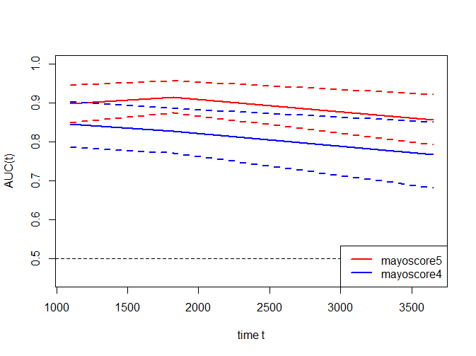
ROC的最佳阈值(cutoff)
一般来说,对于一个biomarker或者简单的说诊断指标/试剂,我们使用ROC曲线计算出AUC值后,还会根据ROC曲线的最佳阈值来确定其灵敏度和特异度,有时在研究中,还会用于KM曲线的分类指标
确定阈值的方法很多(可参考:ROC Curve或者One ROC Curve and Cutoff Analysis),一般会用最常见的约登指数(Youden index),即敏感度+特异性-1;有时也会考虑用其他确定阈值的方法,比如Minimum ROC distance, Misclassification Cost Term等等(参考:ROC)
对于上述timeROC的结果,如3年ROC曲线的约登指数(因为TP代表的是True Positive fraction,即sensitivity;而FP代表的是False Positive fraction,即1-specificity):
> mayo$mayoscore5[which.max(time_ROC_df$TP_3year - time_ROC_df$FP_3year)]
[1] 6.273571
即对于mayoscore5这个marker而言,最佳阈值(cutoff)为6.27
由于医药诊断领域一般是二分类诊断模型,所以上述我们讨论的都是基于二分类的ROC曲线,对于一些特殊情况,还会有多分类的ROC,则不在此之列
参考资料
以上为对于time-dependent ROC的一些小结,主要参考以下资料:
时间依赖性ROC曲线(一)
真实世界大数据分析系列|ROC曲线与Time-dependent ROC 曲线
R|timeROC-TimeDependent ROC分析
One ROC Curve and Cutoff Analysis
ROC Curve
Time-dependent ROC for Survival Prediction Models in R
本文出自于http://www.bioinfo-scrounger.com转载请注明出处