Bland-Altman Analysis

The Bland-Altman analysis is the most common method of assessing the agreement in method comparison in IVD CT or CE trials.

The Bland-Altman method generally refers to the Bland-Altman plot, which is used to display the relationship between two paired quantitative measurement tests or assays (Bland & Altman, 1986 and 1999). For example, a new product might be compared with the registered product, or previous generation product. Alternatively the product can be the reference or gold standard method. Sometimes we would call it a different plot instead of the Bland-Altman plot in the CLSI EP09.

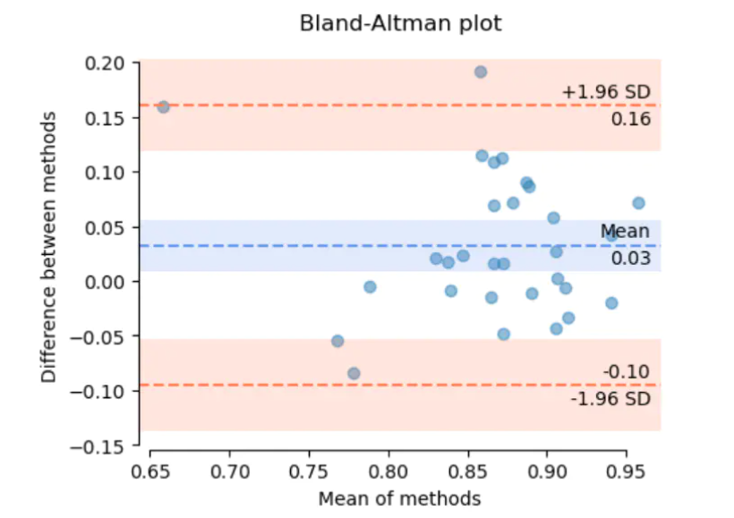
As we can see from above, the Bland-Altman is a scatter plot that clearly shows the relationship between the differences and the magnitude of measurement. The X axis represents the mean of two measurements, and the Y axis represents the difference.

Sometimes the difference can be defined as constant difference, but it also can be defined as proportional difference that depends on the distribution of measurements. For example, if the difference is not related to the magnitude, it means that we have a constant difference between the two assays throughout the total X axis range. Otherwise proportional difference means that it’s related to the magnitude, and proportional to the magnitude. So such plots can be visually inspected to determine the underlying variability characteristic of this relationship.

Assumption

The assumption of Bland-Altman is that the differences are normally distributed. But we all know that we can not make sure the measurements are following the normal distribution completely. In many cases, actually there will not be a big impact for Bland-Altman analysis when the distribution of the differences is not normally distributed.

But from my side, I propose that the range of the two assays should not be too different, be assured that they are in the similar magnitude.

Basics

There have been some definitions we should know for Bland Altman analysis.

Bias, it refers to the mean of the differences of the two measurements. It can be seen in the middle line in the Bland Altman plot, which is useful for detecting a systematic difference.
95% CI of Bias, it refers to the 95% confidence interval of the mean difference, which illustrates the magnitude of the systematic difference.
Limits of Agreement (LoA), it refers to the 95% prediction interval of the differences. And it can be seen in the upper and lower lines in the Bland Altman plot. This indicator is very important in clinical trials. Always we need to compare the LoA with the clinical acceptance criteria to demonstrate the bias for the new product is accepted in clinical practice.
95% CI of LoA, it refers to the 95% confidence interval of LoA, to demonstrate the error or precision of the upper and lower LoA.

Analysis

To explain the calculation process more clearly, here I use the R to implement it.

Suppose you have two measurements from different assays. The mean differences of them is 5, and the corresponding standard deviation is 0.8.

d <- 5
sd <- 0.8

We can easily get the LoA by the formula as it’s the prediction interval of the differences.

LoA <- c(d - 1.96 * sd, d + 1.96 * sd)

And the CI for d and LoA would be a bit complicated, as shown below from NCSS Bland-Altman Plot and Analysis documentation.

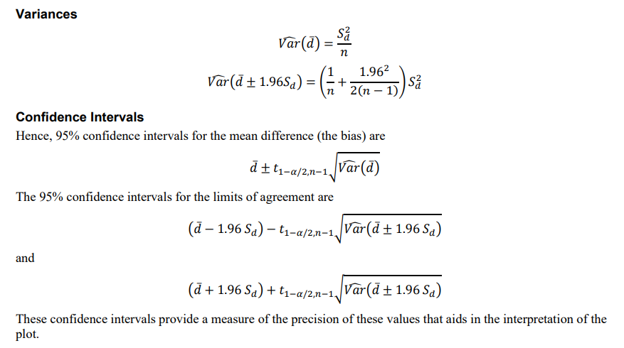
From the above formula, the standard error of LoA CI is about 1.71 times as the d. This 1.71 always occurs in some Bland Altman related articles,for now at least we have known how to calculate this number. Just drop the n from both sides of the equation.

sqrt(1 + 1.96^2 / 2)

For the CI, we can also easily calculate them according to the above formula, for example the 95% two-side confidence interval.

But here we must make sure that we should use the t distribution or normal distribution, that will affect whether we use t statistic or z statistic. Suppose here I use t distribution, and define the sample size n is 200, so degrees of freedom is equal to n-1.

n <- 200
t <- qt(1 - 0.05 / 2, 200-1)

d_se <- sd / sqrt(n)
d_CI <- c(d - t * d_se, d + t * d_se)
> d_CI
[1] 4.888449 5.111551

Then the corresponding CI of LoA

LoA_se <- sd * sqrt(1 / n + 1.96^2 / (2 * (n - 1)))
LoA_CI <- LoA + c(- t * LoA_se, t * LoA_se)
> LoA_CI
[1] 3.241041 6.758959s

Results

What's the best result for Bland Altman analysis in the clinical trials?

Basically in the Bland Altman plot, we hope the spread of the scatter points is consistent across the range of X axis. And only a few points fall outside LoA. Moreover, the LoA or LoA CI meet the clinical requirements.

Reference

Above all are my rough understanding, the main purpose is to note the calculation of CI for LoA. The references are as shown below:

Bland-Altman Plots(一致性评价)在python中的实现
 Bland-Altman Plot and Analysis
Bland-Altman plot
Bland-Altman 分析在临床测量方法一致性评价中的应用

Please indicate the source: http://www.bioinfo-scrounger.com