Hypothesis testing of MMRM

Originally, I created an issue in CAMIS github asking how to do the hypothesis testing of MMRM in R, especially in non-inferiority or superiority trials. And then I received a reminder that I can get the manual from mmrm package document.

The mmrm package has provided the df_1d() function to do the one-dimensional contrast. So let's start by fitting a mmrm model first with us (unstructured) covariance structure and Kenward-Roger adjustment methods. I also include a linear Kenward-Roger approximation for coefficient covariance matrix adjustment so that R results can be compared with SAS when the unstructured covariance model is selected.

library(mmrm)

fit <- mmrm(
  formula = FEV1 ~ RACE + SEX + ARMCD * AVISIT + us(AVISIT | USUBJID),
  reml = TRUE, method = "Kenward-Roger", vcov = "Kenward-Roger-Linear",
  data = fev_data
)
summary(fit)

Assuming that we aim to compare Race white with Race Asian, the results are as follows.

contrast <- numeric(length(component(fit, "beta_est")))
contrast[3] <- 1
df_1d(fit, contrast)

# same as 
# emmeans(fit, ~ RACE) %>% contrast() %>% test()

Honestly, I prefer to use the emmeans package to compute estimated marginal means (least-square means), especially when you also want to compute it by visit and by treatment. Because mmrm package sets an object interface so that it can be used for the emmeans package. And emmeans has also built a set of useful functions to deal with common questions. So it’s a good solution to fit the MMRM model by mmrm and do hypothesis testing by emmeans.

A general assumption is that we would like to compute the least-square means first for the coefficients of the MMRM by visit and by treatment. This can be done through emmeans() and confint() functions.

library(emmeans)

ems <- emmeans(fit, ~ ARMCD | AVISIT)
confint(ems)

## AVISIT = VIS1:
##  ARMCD emmean    SE  df lower.CL upper.CL
##  PBO     33.3 0.761 148     31.8     34.8
##  TRT     37.1 0.767 143     35.6     38.6
## 
## AVISIT = VIS2:
##  ARMCD emmean    SE  df lower.CL upper.CL
##  PBO     38.2 0.616 147     37.0     39.4
##  TRT     41.9 0.605 143     40.7     43.1
## 
## AVISIT = VIS3:
##  ARMCD emmean    SE  df lower.CL upper.CL
##  PBO     43.7 0.465 130     42.8     44.6
##  TRT     46.8 0.513 130     45.7     47.8
## 
## AVISIT = VIS4:
##  ARMCD emmean    SE  df lower.CL upper.CL
##  PBO     48.4 1.199 134     46.0     50.8
##  TRT     52.8 1.196 133     50.4     55.1
## 
## Results are averaged over the levels of: RACE, SEX 
## Confidence level used: 0.95

Naturally we will also want to consider the contrast to see what is the difference between treatment and placebo where the null hypothesis is that treatment minus placebo equals zero. Here the contrast() function will be run. If you want to see the confidence interval of difference, just use confint(contr) that will be fine. PS. You can relevel the order of ARMCD factor in advance, in that case the method=pairwise can reach the same results as well.

contr <- contrast(ems, adjust = "none", method = "revpairwise")
contr

## AVISIT = VIS1:
##  contrast  estimate    SE  df t.ratio p.value
##  TRT - PBO     3.77 1.082 146   3.489  0.0006
## 
## AVISIT = VIS2:
##  contrast  estimate    SE  df t.ratio p.value
##  TRT - PBO     3.73 0.863 145   4.323  <.0001
## 
## AVISIT = VIS3:
##  contrast  estimate    SE  df t.ratio p.value
##  TRT - PBO     3.08 0.696 131   4.429  <.0001
## 
## AVISIT = VIS4:
##  contrast  estimate    SE  df t.ratio p.value
##  TRT - PBO     4.40 1.693 133   2.597  0.0104
## 
## Results are averaged over the levels of: RACE, SEX

Besides maybe we would like to further assess whether treatment is superior to placebo with a margin of 2. You can utilize the test() function with the null = 2 argument.

test(contr, null = 2, side = ">")

## AVISIT = VIS1:
##  contrast  estimate    SE  df null t.ratio p.value
##  TRT - PBO     3.77 1.082 146    2   1.640  0.0516
## 
## AVISIT = VIS2:
##  contrast  estimate    SE  df null t.ratio p.value
##  TRT - PBO     3.73 0.863 145    2   2.007  0.0233
## 
## AVISIT = VIS3:
##  contrast  estimate    SE  df null t.ratio p.value
##  TRT - PBO     3.08 0.696 131    2   1.554  0.0613
## 
## AVISIT = VIS4:
##  contrast  estimate    SE  df null t.ratio p.value
##  TRT - PBO     4.40 1.693 133    2   1.416  0.0795
## 
## Results are averaged over the levels of: RACE, SEX 
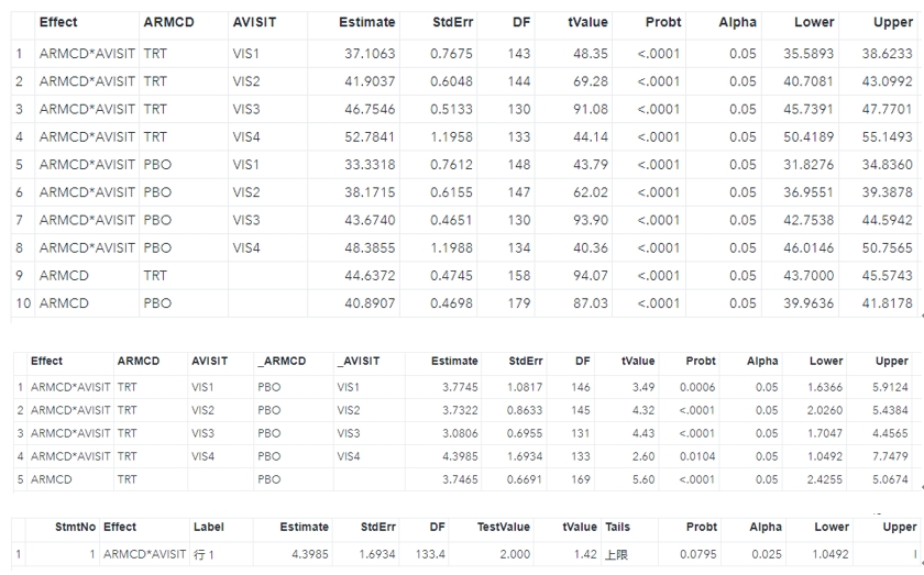
## P values are right-tailed

In general the common estimations and hypothesis testing of MMRM are all here, which at least I have encountered. In the next step, I want to compare the above results with SAS to see if it can be regarded as additional QC validation. We use the lsmeans statement to estimate least-square means and do superiority testing at visit 4 through lsmestimate statement.

proc mixed data=fev_data;
    class ARMCD(ref='PBO') AVISIT RACE SEX USUBJID;
    model FEV1 = RACE SEX ARMCD ARMCD*AVISIT / ddfm=KR;
    repeated AVISIT / subject=USUBJID type=UN r rcorr;
    lsmeans ARMCD*AVISIT / cl alpha=0.05 diff slice=AVISIT;
    lsmeans ARMCD / cl alpha=0.05 diff;
    lsmestimate ARMCD*AVISIT [1,1 4] [-1,2 4] / cl upper alpha=0.025 testvalue=2;
    ods output lsmeans=lsm diffs=diff LSMEstimates=est;
run;

All of the results can be shown below, and they are consistent with the R results.

Reference

MMRM Package Introduction