前段时间逛Kaggle的时候,发现有个对于Covid-19的预测比赛(COVID19 Global Forecasting (Week 4)),其给出的数据有以下几列:
- Province_State,省
- Country_Region,国家
- Date,日期
- ConfirmedCases,确诊人数
- Fatalities,死亡人数 从一些已提交的notebook中可看出,对于此类数据,比较常见的方法是采用SIR模型,再搭配一些机器学习的方法来预测模型的某些参数
SIR是三个单词首字母的缩写,其中S是Susceptible的缩写,表示易感者;I是Infective的缩写,表示感染者;R是Removal的缩写,表示移除者。
最开始的时候,我由于知识的局限性,对于SIR模型属于一头雾水,查了一些国内的中文资料,但理解的不够深入;最后在google上查到一篇文章,个人认为讲的非常详细,在此分享下:SIR models in R,其主要从三部分对SIR的用法进行了讲解:
- Three representations of an SIR model
- Solving differential equations in R
- Estimating model's parameters
常见的一些自媒体的文章一般只讲到上述中的第一点,有些会提到第二点,但是我觉得把第一和第二点连起来看会更加助于理解
以下是小小的搬运工
Three representations of an SIR model
从SIR介绍可看出,S/I/R三者的关系如下,其中两个参数β和γ分别代表感染率和恢复率

将上述三者关系写成微分方程形式:
\[ \frac{dS}{dt} = -\beta \times I \times S \]
\[ \frac{dI}{dt} = \beta \times I \times S - \gamma\times I \]
\[ \frac{dR}{dt} = \gamma\times I \]
则其中基础繁殖数R0等于:
\[ \mbox{R}_0 = \frac{\beta}{\gamma}N \]
Solving differential equations in R
求解上述微分方程,在R中可用deSolve包的ode()函数(对于Python可自行查一下,也有可调用的函数)
首先根据上述微分方程,写成函数形式(用with函数是因为其只能用于列表/数据框,而无法用于向量):
sir_equations <- function(time, variables, parameters) {
  with(as.list(c(variables, parameters)), {
    dS <- -beta * I * S
    dI <-  beta * I * S - gamma * I
    dR <-  gamma * I
    return(list(c(dS, dI, dR)))
  })
}接着我们为了理解ode()函数的用法,先自行定义参数β/γ的初始值以及S/I/R变量的初始值:
parameters_values <- c(
  beta  = 0.004, # infectious contact rate (/person/day)
  gamma = 0.5    # recovery rate (/day)
)

initial_values <- c(
  S = 999,  # number of susceptibles at time = 0
  I =   1,  # number of infectious at time = 0
  R =   0   # number of recovered (and immune) at time = 0
)
指定时间节点,用于计算在此时间节点下SIR模型变量对应的值
time_values <- seq(0, 10) # days然后就可以调用ode()函数对微分方程进行求解
sir_values_1 <- ode(
  y = initial_values,
  times = time_values,
  func = sir_equations,
  parms = parameters_values
)
> sir_values_1
   time           S         I          R
1     0 999.0000000   1.00000   0.000000
2     1 963.7055761  31.79830   4.496125
3     2 461.5687749 441.91575  96.515480
4     3  46.1563480 569.50418 384.339476
5     4   7.0358807 373.49831 619.465807
6     5   2.1489407 230.12934 767.721720
7     6   1.0390927 140.41085 858.550058
8     7   0.6674074  85.44479 913.887801
9     8   0.5098627  51.94498 947.545162
10    9   0.4328913  31.56515 968.001960
11   10   0.3919173  19.17668 980.431400
再看下R0值(从结果得出为8)
> (999 + 1) * parameters_values["beta"] / parameters_values["gamma"]
beta
   8
最后绘制一些常见的SIR模型的曲线图
with(data.frame(sir_values_1), {
  # plotting the time series of susceptibles:
  plot(time, S, type = "l", col = "blue",
       xlab = "time (days)", ylab = "number of people")
  # adding the time series of infectious:
  lines(time, I, col = "red")
  # adding the time series of recovered:
  lines(time, R, col = "green")
})

# adding a legend:
legend("right", c("susceptibles", "infectious", "recovered"),
       col = c("blue", "red", "green"), lty = 1, bty = "n")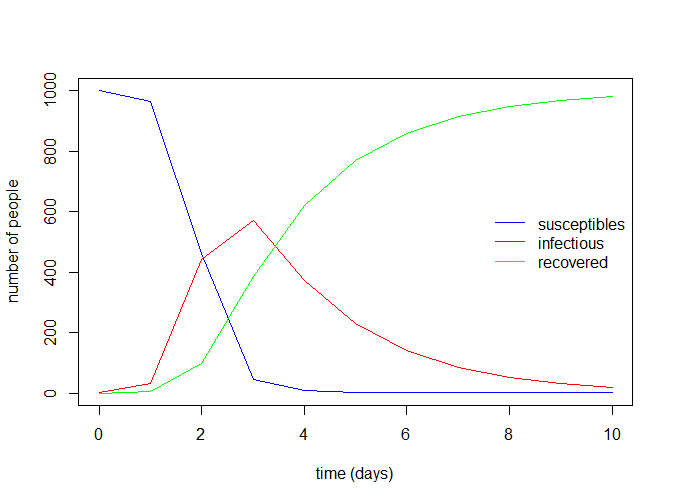
一般的文章/教程到此的结束了,总让的意犹未尽,比如对于上述β/γ参数如何估计等问题都没得到解决;因此需要接着看下一章
Estimating model's parameters
首先将上述过程写到一个预测函数以方便调用
sir_1 <- function(beta, gamma, S0, I0, R0, times) {
  require(deSolve) # for the "ode" function

# the differential equations:
  sir_equations <- function(time, variables, parameters) {
  with(as.list(c(variables, parameters)), {
    dS <- -beta * I * S
    dI <-  beta * I * S - gamma * I
    dR <-  gamma * I
    return(list(c(dS, dI, dR)))
  })
  }

# the parameters values:
  parameters_values <- c(beta  = beta, gamma = gamma)

# the initial values of variables:
  initial_values <- c(S = S0, I = I0, R = R0)

# solving
  out <- ode(initial_values, times, sir_equations, parameters_values)

# returning the output:
  as.data.frame(out)
}
读取文章教程中提到的示例数据
Downloading some flu data from the internet. Context: flu epidemic in an English boys schoolboard (763 boys in total) from January 22nd, 1978 (day 0) to February 4th, 1978 (day 13).
flu <- read.table("https://bit.ly/2vDqAYN", header = TRUE)根据上述示例数据以及预测函数,写一个拟合函数,并绘制拟合曲线
model_fit <- function(beta, gamma, data, N = 763, ...) {
  I0 <- data$cases[1] # initial number of infected (from data)
  times <- data$day   # time points (from data)
# model's predictions:
  predictions <- sir_1(beta = beta, gamma = gamma,   # parameters
                       S0 = N - I0, I0 = I0, R0 = 0, # variables' intial values
                       times = times)                # time points
# plotting the observed prevalences:
  with(data, plot(day, cases, ...))
# adding the model-predicted prevalence:
  with(predictions, lines(time, I, col = "red"))
}
接着简单看下拟合的结果(参数自定义下)
model_fit(beta = 0.004, gamma = 0.5, flu, pch = 19, col = "red", ylim = c(0, 600))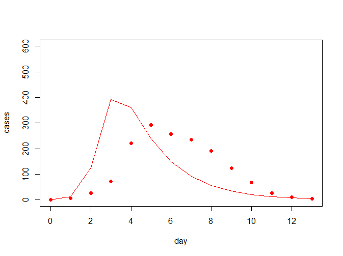
从上图中可看出,拟合曲线跟真实的数据拟合度并不怎么好,因此考虑需要对参数进行一定的估计;常见的我们对于误差的估计会考虑用离差平方和来评估,我们希望提升拟合度就相当于降低离差平方和
将上述计算离差平方和的过程包装到函数中方便调用
ss <- function(beta, gamma, data = flu, N = 763) {
  I0 <- data$cases[1]
  times <- data$day
  predictions <- sir_1(beta = beta, gamma = gamma,   # parameters
                       S0 = N - I0, I0 = I0, R0 = 0, # variables' intial values
                       times = times)                # time points
  sum((predictions$I[-1] - data$cases[-1])^2)
}
对于如何寻找最佳的参数来减少误差,在Machine learning中常见会使用网格搜索(grid search),PS. 当然如果数据集允许的话,可以试下GridSearchCV
在文章教程中,首先使用的是对每个参数在一定值范围内(梯度变化)进行search来约定最佳参数使得离差平方和最小;接着联合考虑两个参数β/γ同时进行search;以上两种相当于在一系列参数值中寻找最佳参数
但是作者还提到可以采用更加有效的方法,比如用optim()函数
Stats中的optim函数是解决优化问题的一个简易的方法,默认是采用Nelder-Mead,具体方法可根据实际情况进行选择
ss2 <- function(x) {
  ss(beta = x[1], gamma = x[2])
}

starting_param_val <- c(0.004, 0.5)
ss_optim <- optim(starting_param_val, ss2)
> ss_optim
$par
[1] 0.002569418 0.475099614

$value
[1] 4799.546

$counts
function gradient
      75       NA

$convergence
[1] 0

$message
NULL从上结果可看出,最佳参数(beta = 0.002569418, gamma = 0.475099614)下,离差平方和最小为4799.546,拟合曲线如下所示:
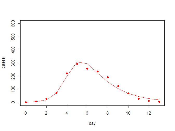
那么此时的R0为R0=763*0.002569418/0.475099614=4.12
Estimating R0
对于R0的估计,还可以用R0包来计算;上述计算R0的方法属于数理计算法
数理计算法,是通过数理模型模拟疾病的发展,再通过模拟的数据计算出R0。理论上来说,只要参数足够精确,数学模型可以比较好地拟合疾病过程。传染病传播动力学模型(SEIR、SIR等)是常用的数理模型。
那么R0包的计算方式属于统计模型计算法
统计模型计算法以概率论为基础,利用疾病的流行曲线对R0进行估计。因该方法基于实际的病例数据,许多研究都利用这种方法计算R0。下面我们采用统计模型计算方法,应用R软件对R0进行估计。
R0包的estimate.R函数来计算R0值,参数比较简单,也有多种methods可选,只是其中有代际时间(Serial interval)的分布需要预先进行估计
如中国疾控中心团队在《新英格兰医学杂志》发表的文章发现,COVID-19的代际时间符合gamma分布,均值、标准差分别为7.5和3.4
那么GTn则为:
GTn <- generation.time(type="gamma", val=c(7.5,3.4))接着使用estimate.R函数来估计R0(由于flu示例数据的代际时间未知,所以使用函数的示例数据)
data(Germany.1918)
mGT<-generation.time("gamma", c(3, 1.5))
estimate.R(Germany.1918, mGT, begin=1, end=27, methods=c("EG", "ML", "TD", "AR", "SB"), pop.size=100000, nsim=100)其实上述这块我也不太能说清楚,不太专业,主要参考:COVID-19专题:关于R0,你想知道的都在这里
Maximum likelihood estimation
最后作者对于β/γ这两个参数的估计方法进一步做了扩展,使用了最大似然估计法(Maximum likelihood estimation)代替前面所用的离差平方和法(sum of squares);所用的R包为bbmle,思路是:
先构建似然函数
mLL <- function(beta, gamma, sigma, day, cases, N = 763) {
  beta <- exp(beta) # to make sure that the parameters are positive
  gamma <- exp(gamma)
  sigma <- exp(sigma)
  I0 <- cases[1] # initial number of infectious
  observations <- cases[-1] # the fit is done on the other data points
  predictions <- sir_1(beta = beta, gamma = gamma,
                       S0 = N - I0, I0 = I0, R0 = 0, times = day)
  predictions <- predictions$I[-1] # removing the first point too
# returning minus log-likelihood:
  -sum(dnorm(x = observations, mean = predictions, sd = sigma, log = TRUE))
}然后用bbmle包的mle2函数进行估计,所用的方法可以跟上述optim函数一样选择Nelder-Mead
starting_param_val <- list(beta = 0.004, gamma = 0.5, sigma = 1)
estimates <- mle2(minuslogl = mLL, start = lapply(starting_param_val, log),
                  method = "Nelder-Mead", data = c(flu, N = 763))
再看下β/γ参数的点估计结果(跟上述离差平方和的结果差不多)
> exp(coef(estimates))
        beta        gamma        sigma
 0.002569489  0.474697037 19.207487576
最后看下拟合曲线,并可查看上述的结果所得的置信区间
N <- 763 # total population size
time_points <- seq(min(flu$day), max(flu$day), le = 100) # vector of time points
I0 <- flu$cases[1] # initial number of infected
param_hat <- exp(coef(estimates)) # parameters estimates
# model's best predictions:
best_predictions <- sir_1(beta = param_hat["beta"], gamma = param_hat["gamma"],
                          S0 = N - I0, I0 = I0, R0 = 0, time_points)$I
# confidence interval of the best predictions:
cl <- 0.95 # confidence level
cl <- (1 - cl) / 2
lwr <- qnorm(p = cl, mean = best_predictions, sd = param_hat["sigma"])
upr <- qnorm(p = 1 - cl, mean = best_predictions, sd = param_hat["sigma"])
# layout of the plot:
plot(time_points, time_points, ylim = c(0, max(upr)), type = "n",
     xlab = "time (days)", ylab = "prevalence")
# adding the predictions' confidence interval:
sel <- time_points >= 1 # predictions start from the second data point
polygon(c(time_points[sel], rev(time_points[sel])), c(upr[sel], rev(lwr[sel])),
        border = NA, col = adjustcolor("red", alpha.f = 0.1))
# adding the model's best predictions:
lines(time_points, best_predictions, col = "red")
# adding the observed data:
with(flu, points(day, cases, pch = 19, col = "red"))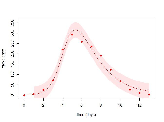
Poisson distribution of errors
从上面的似然函数可看出,其是用了正态分布的密度函数dnorm,这是假设prevelence是符合正态分布的;但我们也可以假设prevelence符合泊松分布( Poisson distributed ),似然函数只需要将sigma改为去掉并且用泊松分布的密度函数qpois即可;处理过程也比较类似,在此就不"复制"代码了,可去看这篇教程的原文
Summary
个人感觉经过这篇教程(https://rpubs.com/choisy/sir)的详细讲解后,让我对于SIR模型有了更好的理解,因此在此推荐给大家;若有看不明白的地方,推荐看原文,效果会更好哈
本文出自于http://www.bioinfo-scrounger.com转载请注明出处