CLSI EP05A3 and EP15A3 as the reference
Definition of Intermediate Precision:
Intermediate precision (also called within-laboratory or within-device) is a measure of precision under a defined set of conditions: same measurement procedure, same measuring system, same location, and replicate measurements on the same or similar objects over an extended period of time. It may include changes to other conditions such as new calibrations, operators, or reagent lots. ——Intermediate precision
Take throwing darts as an example:
- Accuracy: The score you get from the target of darts. The higher the score, the better.
- Precision: The distribution of the score. If you get a very close location, it means your technique is very stable.
Concepts
If you want to estimate the precision for a certain test, these three indicators are useful to figure out whether it’s good enough for using.
- %CV coefficient of variation expressed as a percentage
- %CVR repeatability coefficient of variation
- %CVWL within-laboratory coefficient of variation
We all know that it’s impossible to ensure every test is equal as there are so many factors that would influence our results, such as:
- Day
- Run
- Reagent lot
- Calibrator lot
- Calibration cycle
- Operator
- Instrument
- Laboratory
The first two of the above are usually the main factors to be considered.
Design
So There is always some variants in the measured results compared to real values. It consists of systematic error (bias) and random error. Precision measures random error.
In a single-site 20x2x2 study with 20 days, with two runs per day, with two replicates per run. The associated factors including days and runs will be involved in the statistical analysis, which it used to estimate the two types of precision: repeatability (within-run precision) and within-laboratory precision (within-device precision)
Once the source of variation has been identified, ANOVA model can be used to calculate the SDs and %CVs in the statistical processing of the data. Usual factor can be divided into three components:
Within-run precision (or repeatability), measures the results from replicated samples for a given sample, in a single run, with the essentially constant situation. This variation may be basically caused by random error happening inside the instrument, such as variation of pipetted volumes of sample and reagent.
Between-run precision, measures the variation from different runs (e.g. run1 and run2). This run factor may cause the operation conditions to change, such as temperature, instrument status etc.
Between-day precision, measures the variation happening between days, which is easy to understand, such as caused by humidity etc.
Single Site Precision Evaluation Study
This protocol (20x2x2) is to estimate the repeatability (within-run) and within-laboratory (intermediate precision) following CLSI EP-15.
From the description above, we can find the protocol is a classic nested (hierarchical) design, where replicates are nested within runs and runs are nested within days. So in this situation, nested ANOVA is appropriate. If two factors are involved, corresponding to two-way nested ANOVA.
To estimate the precision of this single-site 20x2x2 design, we should follow a nested linear components-of-variance model involving two factors: “day” and “run”, with “run” nested with “day”. I think this model can be analyzed using the two-way nested ANOVA. It should be noted that the design is balanced because it specifies the same number of runs for each day, and the same number of replicates for each run.
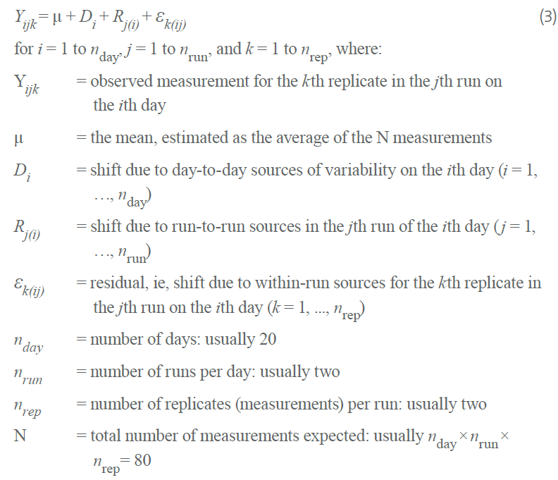
The above screenshot from CLSI EP05-A3 can help us to understand the nested linear components-of-variance model. We can especially know that the residual in the model represents the within-run factor.
Fit a random effects model
Nested random effects are when each member of one group is contained entirely within a single unit of another group. The canonical example is students in classrooms Crossed random effects are when this nesting is not true. An example would be different seeds and different fields used for planting crops. Seeds of the same type can be planted in different fields, and each field can have multiple seeds in it.
Whether random effects are nested or crossed is a property of the data, not the model. In the other word, you should tell the model which data is nested or crossed.
I don’t describe the experiment and workflow in this section, which can be found in the CLSI EP05 and EP15 documents clearly.
Data analysis by ANOVA
Let’s talk about how to calculate the %CV and SD that can be divided into at least two categories based on how many factors are involved.
The first step, I load a simple design(20x2x2) data from a R package VCA including 2 replicates, 2 runs and 20 days from a single sample,where y is the test measurements.
One reagent lot - a single sample
One instrument system
20 test days
Two runs per day
Two replicates measurements per run
library(VCA) data(dataEP05A2_2) > summary(dataEP05A2_2) day run y
1 : 4 1:40 Min. :68.87
2 : 4 2:40 1st Qu.:73.22
3 : 4 Median :75.39
4 : 4 Mean :75.41
5 : 4 3rd Qu.:77.37
6 : 4 Max. :83.02
(Other):56
The second step, I use the nested ANOVA by aov function in R to fit a nested linear components-of-variance model. In this situation, runs are nested within days.
res <- aov(y~day/run, data = dataEP05A2_2)
ss <- summary(res)
> ss
            Df Sum Sq Mean Sq F value  Pr(>F)
day         19  319.0  16.787   4.512   3e-05 ***
day:run     20  187.4   9.372   2.519 0.00634 **
Residuals   40  148.8   3.720
---
Signif. codes:  0 ‘***’ 0.001 ‘**’ 0.01 ‘*’ 0.05 ‘.’ 0.1 ‘ ’ 1
The third step, calculate the SD and %CV of the day, run and error variation following the formula occurred in EP05-A3. By the way, the error CV(CVerror) is corresding to %CVR, also called within-run or repeatability precision. And the %CVWL is the within-laboratory precision.
nrep <- 2
nrun <- 2
nday <- 20
Verror <- ss[[1]]$`Mean Sq`[3]
Vrun <- (ss[[1]]$`Mean Sq`[2] - ss[[1]]$`Mean Sq`[3]) / nrep
Vday <- (ss[[1]]$`Mean Sq`[1] - ss[[1]]$`Mean Sq`[2]) / (nrun * nrep)

Serror <- sqrt(Verror)
Sday <- sqrt(Vday)
Srun <- sqrt(Vrun)
Swl <- sqrt(Vday + Vrun + Verror)
> print(c(Swl, Sday, Srun, Serror))
[1] 2.898293 1.361533 1.681086 1.928803

CVerror <- Serror / mean(dataEP05A2_2$y) * 100
> CVerror
[1] 2.557875
CVwl <- Swl / mean(dataEP05A2_2$y) * 100
> CVwl
[1] 3.843561
The fourth step, calculate the confidence interval of SD and %CV, which is relying on the chi-square distribution value for DF estimates. Use the CV% of error as an example.

alpha <- 0.05
CVCI <- c(CVerror * sqrt(ss[[1]]$Df[3] / qchisq(1-alpha/2, df = 40)), CVerror * sqrt(ss[[1]]$Df[3] / qchisq(alpha/2, df = 40)))
> CVCI
[1] 2.100049 3.272809
CVCI_oneSide <- c(CVerror * sqrt(ss[[1]]$Df[3] / qchisq(1-alpha, df = 40)), CVerror * sqrt(ss[[1]]$Df[3] / qchisq(alpha, df = 40)))
> CVCI_oneSide
[1] 2.166476 3.142029
Fortunately, above standard calculation steps have been packed into a R package, that is the VCA package. So we just apply anovaVCA function to fit the model and summarize the it. For CI calculation, the VCAinference function could be used. It sounds so good.
Fit model:
res <- anovaVCA(y~day/run, dataEP05A2_2)
res
> res


Result Variance Component Analysis:
-----------------------------------

  Name    DF       SS         MS        VC       %Total    SD       CV[%]
1 total   54.78206                      8.400103 100       2.898293 3.843561
2 day     19       318.961943 16.787471 1.853772 22.068447 1.361533 1.805592
3 day:run 20       187.447626 9.372381  2.82605  33.643043 1.681086 2.229366
4 error   40       148.811221 3.720281  3.720281 44.288509 1.928803 2.557875

Mean: 75.40645 (N = 80)

Experimental Design: balanced  |  Method: ANOVA
Calculate CI for SD and %CV:
VCAinference(res)
> VCAinference(res)


Inference from (V)ariance (C)omponent (A)nalysis
------------------------------------------------

> VCA Result:
-------------

  Name    DF      SS       MS      VC     %Total  SD     CV[%]
1 total   54.7821                  8.4001 100     2.8983 3.8436
2 day     19      318.9619 16.7875 1.8538 22.0684 1.3615 1.8056
3 day:run 20      187.4476 9.3724  2.8261 33.643  1.6811 2.2294
4 error   40      148.8112 3.7203  3.7203 44.2885 1.9288 2.5579

Mean: 75.4064 (N = 80)

Experimental Design: balanced  |  Method: ANOVA


> VC:
-----
        Estimate CI LCL  CI UCL One-Sided LCL One-Sided UCL
total     8.4001 5.9669 12.7046        6.2987       11.8680
day       1.8538
day:run   2.8261
error     3.7203 2.5077  6.0906        2.6689        5.6135

> SD:
-----
        Estimate CI LCL CI UCL One-Sided LCL One-Sided UCL
total     2.8983 2.4427 3.5644        2.5097        3.4450
day       1.3615
day:run   1.6811
error     1.9288 1.5836 2.4679        1.6337        2.3693

> CV[%]:
--------
        Estimate CI LCL CI UCL One-Sided LCL One-Sided UCL
total     3.8436 3.2394 4.7269        3.3282        4.5686
day       1.8056
day:run   2.2294
error     2.5579 2.1000 3.2728        2.1665        3.1420


95% Confidence Level
SAS PROC MIXED method used for computing CIs
These functions can be used to handle complicated design, so we don't need to set up functions or a package any more.
Reference
Visualizing Nested and Cross Random Effects
R-Package VCA for Variance Component Analysis
How to Perform a Nested ANOVA in R (Step-by-Step)
Lab 8 - Nested and Repeated Measures ANOVA
What’s with the precision?
Please indicate the source: http://www.bioinfo-scrounger.com