I have a strong interest in data visualization. For me, the purpose to learn this skill is driven by having a good understanding and examination for the question one wants to solve.
The alluvial plot and Sankey diagram are both forms of visualization for general flow diagrams. These plot types are designed to show the change in magnitude of some quantity as it flows between states. Although the difference between alluvial plot and sankey diagram is always discussed online, like the issue Alluvial diagram vs Sankey diagram?, here just comes how to allow us to study the connection and flow of data between different categorical features in R. So we don’t mind the mixed use by both of them.
Note: an Alluvial diagram is a subcategory of Sankey diagrams where nodes are grouped in vertical nodes (sometimes called steps).
For illustrating the following cases, I will load the flight data from nycflights13 library first. This comprehensive data set contains all flights that departed from the New York City airports JFK, LGA and EWR in 2013, including three columns we’re concerned about, such as origin (airport of origin), dest (destination airport) and carrier (airline code). For a better demonstration, I select the top five destinations and top four carriers.
top_dest <- flights %>%
  count(dest) %>%
  top_n(5, n) %>%
  pull(dest)

top_carrier <- flights %>%
  filter(dest %in% top_dest) %>%
  count(carrier) %>%
  top_n(4, n) %>%
  pull(carrier)

fly <- flights %>%
  filter(dest %in% top_dest & carrier %in% top_carrier)
Let‘s take a look at the sankey, Google defines a sankey as:
A sankey diagram is a visualization used to depict a flow from one set of values to another. The things being connected are called nodes and the connections are called links. Sankeys are best used when you want to show a many-to-many mapping between two domains or multiple paths through a set of stages.
In R, we can plot a sankey diagram with the ggsankey package in the ggplot2 framework. This package is very kind to provide a function (make_long()) to transform our common wide data to long.
fly <- flights %>%
  filter(dest %in% top_dest & carrier %in% top_carrier) %>%
  ggsankey::make_long(origin, carrier, dest)
In R, we can plot a sankey diagram with the ggsankey package in the ggplot2 framework. This package is very kind to provide a function (make_long()) to transform our common wide data to long, so that columns will be fit to the parameters in functions. It contains four columns, corresponding to stage and node, such as stage is for x and next_x, and node is for node and next_node. Hence, at least four columns are required. More usages are illustrated in this document(https://github.com/davidsjoberg/ggsankey).
So a basic sankey diagram is as following:
ggplot(fly, aes(x = x, next_x = next_x,
                node = node, next_node = next_node,
                fill = factor(node), label = node)) +
  geom_sankey(flow.alpha = 0.6, node.color = "gray30") +
  geom_sankey_label(size = 3, color = "white", fill = "gray40") +
  scale_fill_viridis_d() +
  theme_sankey(base_size = 18) +
  labs(x = NULL) +
  theme(legend.position = "none",
        plot.title = element_text(hjust = .5))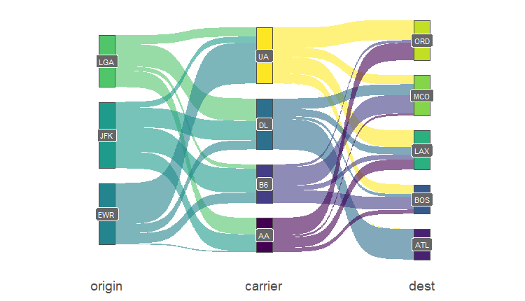
Furthermore, networkD3 package is also able to plot the sankey diagram, but not easy to use I think.
After my initial use, alluvial and ggalluvial packages are very suitable for R users to create the alluvial plots. The former has its own specific syntax, otherwise the later one can be integrated seamlessly into ggplot2, same as ggsankey.
Actually, to be honest, both of them are convenient. You can choose either one according to your use situation. For example, thealluvial package is demonstrated below:
fly <- flights %>%
  filter(dest %in% top_dest & carrier %in% top_carrier) %>%
  count(origin, carrier, dest) %>%
  mutate(origin = fct_relevel(as.factor(origin), c("EWR","JFK","LGA")))
alluvial(fly %>% select(-n),
         freq = fly$n, border = NA, alpha = 0.5,
         col=case_when(fly$origin == "JFK" ~ "red",
                       fly$origin == "EWR" ~ "blue",
                       TRUE ~ "orange"),
         cex = 0.75,
         axis_labels = c("Origin", "Carrier", "Destination"))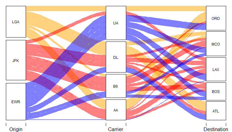
The detailed usages can be found in this web (https://github.com/mbojan/alluvial).
If you would like to own more customized adjustments, maybe the ggsankey is better. As it’s a ggplot2 extension, which has enough functions for modification following your thoughts.
We still don’t need to take much time to transform data because ggalluvial also has a very convenient function to do the same procedure as make_long() in ggsankey. If your data is in a “wide” format , like the flight dataset, the to_lodes_form() function will help you easily.
fly <- flights %>%
  filter(dest %in% top_dest & carrier %in% top_carrier) %>%
  count(origin, carrier, dest) %>%
  mutate(
    origin = fct_relevel(as.factor(origin), c("LGA", "EWR","JFK")),
    col = origin
  ) %>%
  ggalluvial::to_lodes_form(key = type, axes = c("origin", "carrier", "dest"))
ggplot(data = fly, aes(x = type, stratum = stratum, alluvium = alluvium, y = n)) +
  # geom_lode(width = 1/6) +
  geom_flow(aes(fill = col), width = 1/6, color = "darkgray",
            curve_type = "cubic") +
  # geom_alluvium(aes(fill = stratum)) +
  geom_stratum(color = "grey", width = 1/6) +
  geom_label(stat = "stratum", aes(label = after_stat(stratum))) +
  theme(
    panel.background = element_blank(),
    axis.text.y = element_blank(),
    axis.text.x = element_text(size = 15, face = "bold"),
    axis.title = element_blank(),
    axis.ticks = element_blank(),
    legend.position = "none"
  ) +
  scale_fill_viridis_d()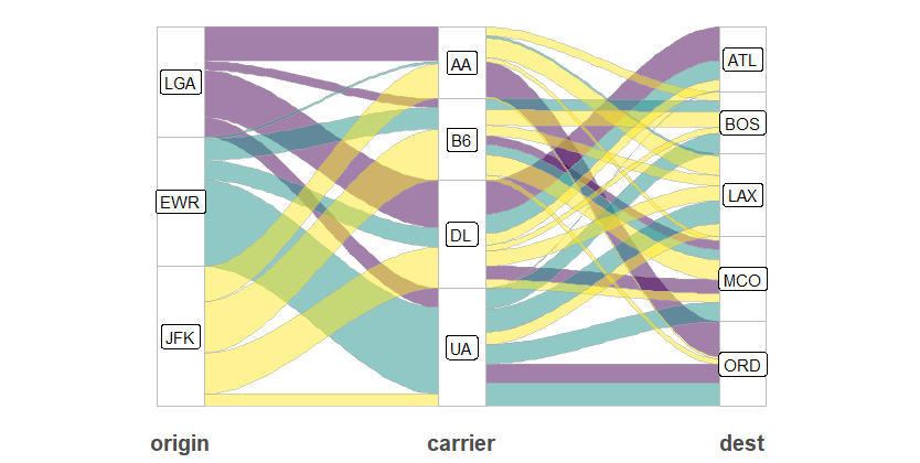
The geom_alluvium() is a bit different to geom_flow(), which is chosen to use depending on the type of dataset you provide and the purpose you want to demonstrate.
Above all are my notes for a previous question. If you have any questions, please read the references as follows, which is easier to understand.
Reference
https://github.com/davidsjoberg/ggsankey
https://www.displayr.com/sankey-diagrams-r/
https://cran.r-project.org/web/packages/alluvial/vignettes/alluvial.html
https://corybrunson.github.io/ggalluvial/
https://www.r-bloggers.com/2019/06/data-flow-visuals-alluvial-vs-ggalluvial-in-r/
https://cran.rstudio.com/web/packages/ggalluvial/vignettes/ggalluvial.html
Please indicate the source: http://www.bioinfo-scrounger.com