Introduction
There are plenty of methods that could be applied to the missing data, depending on the goal of the clinical trial. The most common and recommended is multiple imputation (MI), and other methods such as last observation carried forward (LOCF), observed case (OC) and mixed model for repeated measurement (MMRM) are also available for sensitivity analysis.
Multiple imputation is a model based method, but it's not just the model to impute data, it's also a framework with the implementation of various analytic models like ANCOVA. In general, there are 3 steps to implement MI, where R and SAS are all the same.
- Imputation, generating M datasets with imputed. But before starting this step, you'd better examine the missing pattern, Monotone missing data pattern, or Arbitrary pattern of missing data.
- Analysis, generating M sets of estimates from M imputed datasets using the statistical model.
- Pooling, the M sets of estimates will be combined into one MI estimate. This is very different from other imputation methods as it not only imputes missing values but also outputs the estimated value from multiple imputed datasets. The pooling method is Rubin's Rules (RR), which can pool parameter estimates such as mean differences, regression coefficients and standard errors, and then derive confidence intervals and p-values. The pool logic will be briefly introduced below.
After the routine introduction of MI, let's talk about how to implement the MI model to deal with actual missing data in SAS. I'm also planning to compare the SAS procedure with the rbmi R package in the next article. To be honest, I tend to use R instead of SAS in my actual work, so I would like to introduce more R use in clinical trials.
Implementation
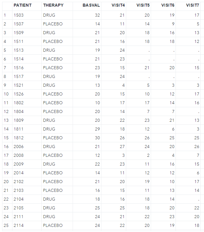
Here is an example dataset from an antidepressant clinical trial of an active drug versus placebo. The relevant endpoint is the Hamilton 17-item depression rating scale (HAMD17) which was assessed at baseline and at weeks 1, 2, 4, and 6. This example comes from the rbmi package so that I can use the same dataset in R programming. But I do the pre-processing and transposing to meet the data type of the MI procedure in SAS.
library(rbmi)
library(tidyverse)

data("antidepressant_data")
dat <- antidepressant_data

# Use expand_locf to add rows corresponding to visits with missing outcomes to the dataset
dat <- expand_locf(
  dat,
  PATIENT = levels(dat$PATIENT), # expand by PATIENT and VISIT
  VISIT = levels(dat$VISIT),
  vars = c("BASVAL", "THERAPY"), # fill with LOCF BASVAL and THERAPY
  group = c("PATIENT"),
  order = c("PATIENT", "VISIT")
)

dat2 <- pivot_wider(
  dat,
  id_cols = c(PATIENT, THERAPY, BASVAL),
  names_from = VISIT,
  names_prefix = "VISIT",
  values_from = HAMDTL17
)
write.csv(dat2, file = "./antidepressant.csv", na = "", row.names = F)
And then import the csv file into SAS, as shown below.
Next, we should examine the missing pattern in the dataset by using zero imputation (nimpute=0).
proc mi data=antidepressant nimpute=0;
    var BASVAL VISIT4 VISIT5 VISIT6 VISIT7;
run;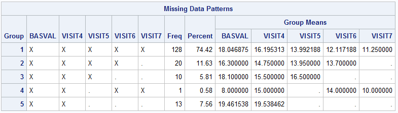
The above graph indicates that there is a patient who doesn’t fit the monotone missing data pattern, so the missing pattern is non-monotone. With regard to which MI method should be performed, the MISSING DATA PATTERNS section and Table 4 from this article(MI FOR MI, OR HOW TO HANDLE MISSING INFORMATION WITH MULTIPLE IMPUTATION) can be used as references. I will select the MCMC (Markov Chain Monte Carlo) method for the multiple imputation afterwards.
Then starting the first step, here I choose the MCMC full-data imputation with impute=full and specify the BY statement to obtain the separate imputed datasets in the treatment group. And I also specify the seed number as well, but keep in mind that it is only defined in the first group; the second group is not the seed number you define but another fixed and random seed number following the seed number you have.
proc sort data=antidepressant; by THERAPY; run;
proc mi data=antidepressant seed=12306 nimpute=100 out=imputed_data;
    mcmc chain=single impute=full initial=em (maxiter=1000) niter=1000 nbiter=1000;
    em maxiter=1000;
    by THERAPY;
    var BASVAL VISIT4 VISIT5 VISIT6 VISIT7;
run;
The second step is to implement the analysis model for each imputation datasets that were created from the first step. Assume that I want to estimate the endpoint of change from baseline at week 6 with the LSmean in each treatment by ANCOVA model, and the difference between them. It will include the fixed effect of treatment and fixed covariate of baseline.
data imputed_data2;
    set imputed_data;
    CHG = VISIT7 - BASVAL;
run;
proc sort; by _imputation_; run;

ods output lsmeans=lsm diffs=diff;
proc mixed data=imputed_data2;
    by _imputation_;
    class THERAPY;
    model CHG=BASVAL THERAPY /ddfm=kr;
    lsmeans THERAPY / cl pdiff diff;
run;
We can see the LS mean for each imputation (_Imputation_) in the lsm dataset where each imputation has two rows including drug and placebo, and the difference between two groups in the diff dataset as shwon below.
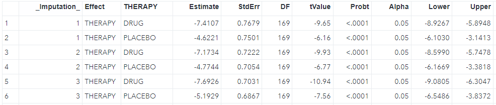

The third step is to pool all estimates from the second step, including the LS mean estimates and difference.
proc sort data=lsm; by THERAPY; run;
ods output ParameterEstimates=combined_lsm;
proc mianalyze data=lsm;
    by THERAPY;
    modeleffects estimate;
    stderr stderr;
run;

ods output ParameterEstimates=combined_diff;
proc mianalyze data=diff;
    by THERAPY _THERAPY;
    modeleffects estimate;
    stderr stderr;
run;
For now the imputations have been combined as shown below.


Above results indicate that each imputation has been combined and the final estimate is calculated by the Rubin's Rules (RR). The t-statistic, confidence interval and p-value are based on t distribution, so the most important is how to calculate the estimate and standard error. The pooled estimate is the mean value of all imputation's estimates. And the pooled SE is the square root of Vtotalthat can be calculated through formulas of 9.2-9.4. The formulas is cited from https://bookdown.org/mwheymans/bookmi/rubins-rules.html.

I'm trying to illustate the computing process of RR in R with the diff dataset as example. Using R is as it's easy for me to do the matrix operations.
diff <- haven::read_sas("./diff.sas7bdat")

est <- mean(diff$Estimate)
> est
[1] -2.803439

n <- nrow(diff)
Vw <- mean(diff$StdErr^2)
Vb <- sum((diff$Estimate - est)^2) / (n - 1)
Vtotal <- Vw + Vb + Vb / n
se <- sqrt(Vtotal)
> se
[1] 1.123403
This est and se value is equal to the pooled Estimate of -2.803439 and StdErr of 1.123403 in SAS.
With the interest of other parameters, you may ask how are the DF and t-statistics calculated? I recommend reading the entire article as mentioned above to comprehend the complete process that is not introduced here. Once the DF and t-statistics are determined, the confidence interval and p-value can be also computed easily by T distribution.
Conclusion
Multiple imputation is a recommended and useful tool in trial use, which provides robust parameter estimates depending on which missing pattern your data has.
In the next article, I will try to illustrate how to use MI in non-inferiority and superiority trials.
Reference
Multiple Imputation using SAS and R Programming
MI FOR MI, OR HOW TO HANDLE MISSING INFORMATION WITH MULTIPLE IMPUTATION
Chapter9 Rubin's Rules