This article is to illustate how to conduct an (Analysis of Covariance) ANCOVA model to determine whether or not the change from baseline glucose is affected by treatment significantly. In other words, using ANCOVA to compare the adjusted means of two or more independent groups while acounting for one or more covariates.
As an example dataset, I'll use the cdiscpilot01 from CDSIC that contains the AdaM and SDTM datasets for a single study. And then our purpose is to conduct efficacy analysis by ANCOVA with LS mean estimation. Suppose that we want to know whether or not the treatment has an impact on Glucose while accounting for the baseline of glucose. The patients are limited to who reach the visit of end of treatment but have not been discontinued due to AE.
Assumptions
ANCOVA makes several assumptions about the input data, such as:
- Linearity between the covariate and the outcome variable
- Homogeneity of regression slopes
- The outcome variable should be approximately normally distributed
- Homoscedasticity
- No significant outliers
Maybe we need to additional article to talk about how to conduct these assumptions, but not in here. So we suppose that all assumptions have been met for the ANCOVA.
Data preparation
Install and load the following required packages. And then load adsl and adlbc datasets from cdiscpilot01 study, which can be referred to another article: Example of SDTM and ADaM datasets from the CDISC.
library(tidyverse)
library(emmeans)
library(gtsummary)
library(multcomp)

adsl <- haven::read_xpt(file = "./phuse-scripts/data/adam/cdiscpilot01/adsl.xpt")
adlb <- haven::read_xpt(file = "./phuse-scripts/data/adam/cdiscpilot01/adlbc.xpt")
Data manipulation
Per the purpose, we need to filter the efficacy population and focus on Glucose (mg/dL) lab test.
gluc <- adlb %>%
  left_join(adsl %>% select(USUBJID, EFFFL), by = "USUBJID") %>%
  # PARAMCD is parameter code and here we focus on Glucose (mg/dL)
  filter(EFFFL == "Y" & PARAMCD == "GLUC") %>%
  arrange(TRTPN) %>%
  mutate(TRTP = factor(TRTP, levels = unique(TRTP)))
And then to produce the analysis datasets by filtering the target patients who have reach out the end of treatment and not been discontinued due to AE.
ana_dat <- gluc %>%
  filter(AVISIT == "End of Treatment" & DSRAEFL == "Y") %>%
  arrange(SUBJID, AVISITN) %>%
  mutate(AVISIT = factor(AVISIT, levels = unique(AVISIT)))
Summary of analysis datsets
Once we have the datasets for analysis, we need to examine the datasets first. I find tbl_summary function in gtsummary package can calculate descriptive statistics and provide a very nice table with clinical style, as shown below:
ana_dat %>%
  dplyr::select(AGEGR1, SEX, RACE, TRTP, AVAL, BASE, CHG) %>%
  tbl_summary(by = TRTP, missing = "no") %>%
  add_n() %>%
  as_gt() %>%
  gt::tab_source_note(gt::md("*This data is from cdiscpilot01 study.*"))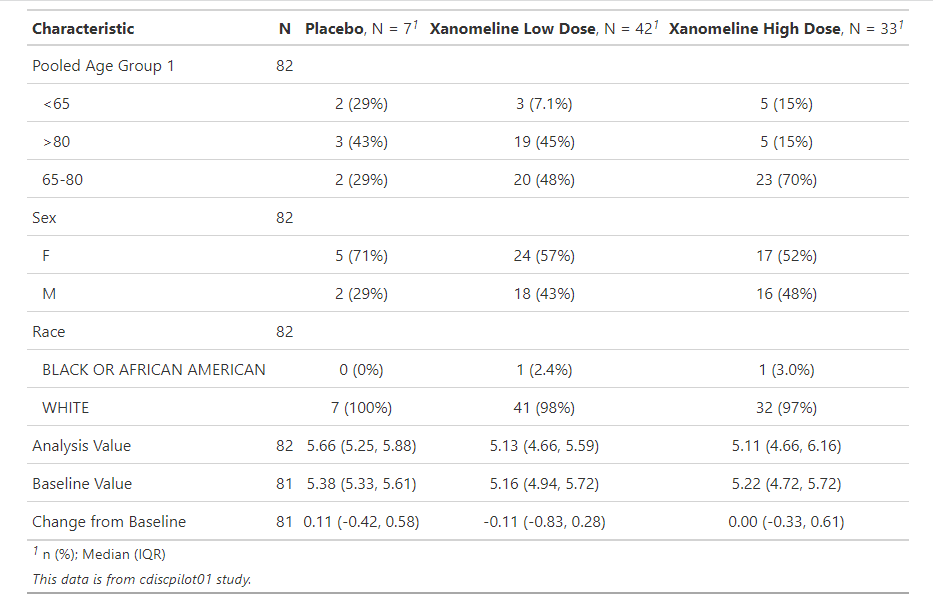
Here we can see the descriptive summary for each variables by the treatment group. Certainly we can also do some visualization like boxplot or scatterplot, but not present here.
Fit ANCOVA model
We use lm function to fit ANCOVA model with treatment(TRTP) as independent variable, change from baseline(CHG)as response variable, and baseline(BASE) as covariates.
fit <- lm(CHG ~ BASE + TRTP, data = ana_dat)
summary(fit)
The summary output for regression coefficients as follows. If you would like to obtain anova tables, should use anova(fit) instead of summary(fit).
Call:
lm(formula = CHG ~ BASE + TRTP, data = ana_dat)

Residuals:
    Min      1Q  Median      3Q     Max
-3.1744 -0.7627 -0.0680  0.5633  5.0349

Coefficients:
                         Estimate Std. Error t value Pr(>|t|)
(Intercept)               -0.5579     0.8809  -0.633    0.528
BASE                       0.1111     0.1329   0.837    0.405
TRTPXanomeline Low Dose   -0.2192     0.5433  -0.404    0.688
TRTPXanomeline High Dose   0.4447     0.5528   0.804    0.424

Residual standard error: 1.328 on 77 degrees of freedom
  (1 observation deleted due to missingness)
Multiple R-squared:  0.06702,   Adjusted R-squared:  0.03068
F-statistic: 1.844 on 3 and 77 DF,  p-value: 0.1462
From above results, we can easily conclude the regression coefficient and model, and the significance comparing to zero. With the coefficient, we can predict the any change based on baseline and treatment.
Besides we can use contrasts function to obtain contrast metrices so that understand the dummy variables for TRTP in the multiple regression model here.
> contrasts(ana_dat$TRTP)
                     Xanomeline Low Dose Xanomeline High Dose
Placebo                                0                    0
Xanomeline Low Dose                    1                    0
Xanomeline High Dose                   0                    1
From the anova table as shown below, it can been seen that the treatment have no statistical significance for the change in glucose under the control of the effects of baseline.
> anova(fit)
Analysis of Variance Table

Response: CHG
          Df  Sum Sq Mean Sq F value Pr(>F)
BASE       1   1.699  1.6989  0.9629 0.3295
TRTP       2   8.061  4.0304  2.2844 0.1087
Residuals 77 135.853  1.7643
If you would like to make the output more pretty, tbl_regression(fit) can be used as mentioned before.
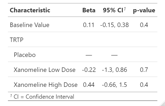
If we want to obtain the least square(LS) mean between treatment groups, emmeans or multcomp package can provide the same results. In addition the process to calculate the LS mean is also very worth to leaning and understanding.
# by multcomp
postHocs <- glht(fit, linfct = mcp(TRTP = "Tukey"))
summary(postHocs)
# by emmeans
fit_within <- emmeans(fit, "TRTP")
pairs(fit_within, reverse = TRUE)
The summary output as shown below:
> summary(postHocs)

     Simultaneous Tests for General Linear Hypotheses

Multiple Comparisons of Means: Tukey Contrasts


Fit: lm(formula = CHG ~ BASE + TRTP, data = ana_dat)

Linear Hypotheses:
                                                Estimate Std. Error t value Pr(>|t|)
Xanomeline Low Dose - Placebo == 0               -0.2192     0.5433  -0.404   0.9116
Xanomeline High Dose - Placebo == 0               0.4447     0.5528   0.804   0.6937
Xanomeline High Dose - Xanomeline Low Dose == 0   0.6639     0.3113   2.132   0.0855 .
---
Signif. codes:  0 ‘***’ 0.001 ‘**’ 0.01 ‘*’ 0.05 ‘.’ 0.1 ‘ ’ 1
(Adjusted p values reported -- single-step method)
Now it's clear a significant difference was observed between the pairs Low Dose vs. Placebo, High Dose vs. Placebo, and High Dose vs. Low Dose.
Reference
https://r4csr.org/efficacy-table.html#efficacy-table
ANCOVA in R
How to perform ANCOVA in R
An Introduction to ANCOVA (Analysis of Variance)
How to Conduct an ANCOVA in R