整理下最近看的生存分析的资料
生存分析是研究生存时间的分布规律,以及生存时间和相关因素之间关系的一种统计分析方法
其主要应用领域:
Cancer studies for patients survival time analyses(临床癌症上病人生存分析)
Sociology for "event-history analysis"(我也不懂)
engineering for "failure-time analysis"(类似于机器使用寿命,故障等研究) 在癌症研究中,其典型研究问题则有:
What is the impact of certain clinical characteristics on patient’s survival(某些临床特征对病人的影响有哪些)
What is the probability that an individual survives 3 years?(病人个体三年存活率有多少)
Are there differences in survival between groups of patients?(两组病人之间的生存率有什么差异)
生存分析使用的方法:
- Kaplan-Meier plots to visualize survival curves(根据生存时间分布,估计生存率以及中位生存时间,以生存曲线方式展示,从而分析生存特征,一般用Kaplan-Meier法,还有寿命法)
- Log-rank test to compare the survival curves of two or more groups(通过比较两组或者多组之间的的生存曲线,一般是生存率及其标准误,从而研究之间的差异,一般用log rank检验)
- Cox proportional hazards regression to describe the effect of variables on survival(用Cox风险比例模型来分析变量对生存的影响,可以两个及两个以上的因素,很常用)
所以一般做生存分析,可以用KM(Kaplan-Meier)方法估计生存率,做生存曲线,然后可以根据分组检验一下多组间生存曲线是否有显著的差异,最后用Cox风险比例模型来研究下某个因素对生存的影响
基本术语:
- Event(事件):在癌症研究中,事件可以是Relapse,Progression以及Death
- Survival time(生存时间):一般指某个事件的开始到终止这段事件,如癌症研究中的疾病确诊到缓解或者死亡,其中有几个比较重要的肿瘤临床试验终点:
- OS(overall survival):指从开始到任意原因死亡的时间,我们一般见到的5年生存率、10年生存率都是基于OS的
- progression-free survival(PFS,无进展生存期):指从开始到肿瘤发生任意进展或者发生死亡的时间;PFS相比OS包含了恶化这个概念,可用于评估一些治疗的临床效益
- time to progress(TTP,疾病进展时间):从开始到肿瘤发生任意进展或者进展前死亡的时间;TTP相比PFS只包含了肿瘤的恶化,不包含死亡
- disease-free survival(DFS,无病生存期):指从开始到肿瘤复发或者任何原因死亡的时间;常用于根治性手术治疗或放疗后的辅助治疗,如乳腺癌术后内分泌疗法等:
- event free survival(EFS,无事件生存期):指从开始到发生任何事件的时间,这里的事件包括肿瘤进展,死亡,治疗方案的改变,致死副作用等(主要用于病程较长的恶性肿瘤、或该实验方案危险性高等情况下)
- Censoring(删失):这经常会在临床资料中看到,生存分析中也有其对应的参数,一般指不是由死亡引起的的数据丢失,可能是失访,可能是非正常原因退出,可能是时间终止而事件未发等等,一般在展示时以‘+’号显示
- left censored(左删失):只知道实际生存时间小于观察到的生存时间
- right censored(右删失):只知道实际生存时间大于观察到的生存时间
- interval censored(区间删失):只知道实际生存时间在某个时间区间范围内
我们前面了解到生存分析需要计算生存率,而生存率(survival rate)则可以看作条件生存概率(conditional probability of survival)的累积,比如三年生存率则是第1-3年每年存活概率的乘积
生存分析的方法一般可以分为三类:
- 参数法:知道生存时间的分布模型,然后根据数据来估计模型参数,最后以分布模型来计算生存率
- 非参数法:不需要生存时间分布,根据样本统计量来估计生存率,常见方法Kaplan-Meier法(乘积极限法)、寿命法
- 半参数法:也不需要生存时间的分布,但最终是通过模型来评估影响生存率的因素,最为常见的是Cox回归模型
而生存曲线(survival curve)则是将每个时间点的生存率连接在一起的曲线,一般随访时间为X轴,生存率为Y轴;曲线平滑则说明高生存率,反之则低生存率;中位生存率(median survival time)越长,则说明预后较好
简单看下Kaplan-Meier方法是怎么计算的:
S(ti)=S(ti−1)(1−di/ni)
- S(ti−1)指在ti−1年还存活的概率
- ni指在在ti年之前还存活的人数
- di指在事件发生的人数
- t0=0,S(0)=1
如果想更加通俗的了解生存率/生存曲线/乘积极限法等概念,可以看画说统计 | 生存分析之Kaplan-Meier曲线都告诉我们什么,比教科书版的解释通俗易懂多啦
最后来看下如何用R来做生存分析
先加载必要的两个包
library("survival")
library("survminer")
使用R包自带的测试数据
data("lung")
> head(lung)
  inst time status age sex ph.ecog ph.karno pat.karno meal.cal wt.loss
1    3  306      2  74   1       1       90       100     1175      NA
2    3  455      2  68   1       0       90        90     1225      15
3    3 1010      1  56   1       0       90        90       NA      15
4    5  210      2  57   1       1       90        60     1150      11
5    1  883      2  60   1       0      100        90       NA       0
6   12 1022      1  74   1       1       50        80      513       0
列名分别是(抄一下了):
* inst: Institution code
* time: Survival time in days
* status: censoring status 1=censored, 2=dead
* age: Age in years
* sex: Male=1 Female=2
* ph.ecog: ECOG performance score (0=good 5=dead)
* ph.karno: Karnofsky performance score (bad=0-good=100) rated by physician
* pat.karno: Karnofsky performance score as rated by patient
* meal.cal: Calories consumed at meals
* wt.loss: Weight loss in last six months接着用Surv()函数创建生存数据对象(主要输入生存时间和状态逻辑值),再用survfit()函数对生存数据对象拟合生存函数,创建KM(Kaplan-Meier)生存曲线
fit <- survfit(Surv(time, status) ~ sex, data = lung)
> print(fit)
Call: survfit(formula = Surv(time, status) ~ sex, data = lung)

        n events median 0.95LCL 0.95UCL
sex=1 138    112    270     212     310
sex=2 90 53 426 348 550如果想看整体的fit结果,可以summary(fit) or summary(fit)$table,但是想看每个时间点的更好的方式则是:
res.sum <- surv_summary(fit)
> head(res.sum)
  time n.risk n.event n.censor      surv    std.err     upper     lower strata sex
1   11    138       3        0 0.9782609 0.01268978 1.0000000 0.9542301  sex=1   1
2   12    135       1        0 0.9710145 0.01470747 0.9994124 0.9434235  sex=1   1
3   13    134       2        0 0.9565217 0.01814885 0.9911586 0.9230952  sex=1   1
4   15    132       1        0 0.9492754 0.01967768 0.9866017 0.9133612  sex=1   1
5   26    131       1        0 0.9420290 0.02111708 0.9818365 0.9038355  sex=1   1
6   30    130       1        0 0.9347826 0.02248469 0.9768989 0.8944820  sex=1   1
具体每个列的含义如下(再抄一下):
* time: the time points on the curve.
* n.risk: the number of subjects at risk at time t
* n.event: the number of events that occurred at time t.
* n.censor: the number of censored subjects, who exit the risk set, without an event, at time t.
* surv: estimate of survival probability.
* std.err: standard error of survival.
* upper: upper end of confidence interval
* lower: lower end of confidence interval
* strata: indicates stratification of curve estimation. If strata is not NULL, there are multiple curves in the result. The levels of strata (a factor) are the labels for the curves.根据上述fit结果,我们可以将KM生存数据进行可视化,主要使用Survminer包的ggsurvplot()函数,如下(这里我们在survfit()函数时用性别因子进行了分组,所以生存曲线有两组,即两条曲线;如果不想分组,将sex换成1即可):
ggsurvplot(fit,
       pval = TRUE, conf.int = TRUE,
       risk.table = TRUE, # Add risk table
       risk.table.col = "strata", # Change risk table color by groups
       linetype = "strata", # Change line type by groups
       surv.median.line = "hv", # Specify median survival
       ggtheme = theme_bw(), # Change ggplot2 theme
       palette = c("#E7B800", "#2E9FDF")
       )
如果想对上图再进行自定义修改,看下ggsurvplot函数说明即可
如果在参数里加上fun = "event"则可绘制cumulative events图(fun除了even外,还有log:log transformation和cumhaz:cumulative hazard)
ggsurvplot(fit,
      conf.int = TRUE,
      risk.table.col = "strata", # Change risk table color by groups
      ggtheme = theme_bw(), # Change ggplot2 theme
      palette = c("#E7B800", "#2E9FDF"),
      fun = "event")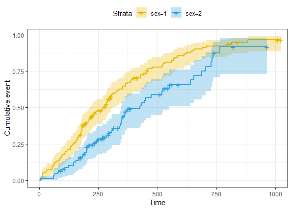
最后如果想对不同组的生存率进行假设检验(Log-Rank test)的话,可以用survdiff()函数,Log-Rank test是无参数检验,近似于卡方检验,零假设是组间没有差异
surv_diff <- survdiff(Surv(time, status) ~ sex, data = lung)
> surv_diff
Call:
survdiff(formula = Surv(time, status) ~ sex, data = lung)

        N Observed Expected (O-E)^2/E (O-E)^2/V
sex=1 138      112     91.6      4.55      10.3
sex=2  90       53     73.4      5.68      10.3

 Chisq= 10.3  on 1 degrees of freedom, p= 0.001
不仅从图中可看出性别组间生存曲线是有差异的,也从Log-Rank test的P值0.001也可得出性别组有显著差异
参考资料:
Survival Analysis Basics
生存分析
生存分析(survival analysis)
本文出自于http://www.bioinfo-scrounger.com转载请注明出处